Our goal in this series is to gain a better understanding of how DeepMind constructed a learning machine — AlphaGo — that was able beat a worldwide Go master. In the first article, we discussed why AlphaGo’s victory represents a breakthrough in computer science. In the the second article, we attempted to demystify machine learning (ML) in general, and reinforcement learning (RL) in particular, by providing a 10,000-foot view of traditional ML and unpacking the main components of an RL system. We discussed how RL agents operate in a flowchart-like world represented by a Markov Decision Process (MDP), and how they seek to optimize their decisions by determining which action in any given state yields the most cumulative future reward. We also defined two important functions, the state-value function (represented mathematically as V) and the action-value function (represented as Q), that RL agents use to guide their actions. In this article, we’ll put all the pieces together to explain how a self-learning algorithm works.
The state-value and action-value functions are the critical bits that makes RL tick. These functions quantify how much each state or action is estimated to be worth in terms of its anticipated, cumulative, future reward. Choosing an action that leads the agent to a state with a high state-value is tantamount to making a decision that maximizes long-term reward — so it goes without saying that getting these functions right is critical. The challenge is, however, that figuring out V and Q is difficult. In fact, one of the main areas of focus in the field of reinforcement learning is finding better and faster ways to accomplish this.
One challenge faced when calculating V and Q is that the value of a given state, let’s say state A, is dependent on the value of other states, and the values of these other states are in turn dependent on the value of state A. This results in a classic chicken-or-the-egg problem: The value of state A depends on the value of state B, but the value of state B depends on the value of state A. It’s circular logic.
Another challenge is that in a stochastic system (in which the results of the actions we take are determined somewhat randomly), when we don’t know the underlying probabilities, the reward that an agent receives when following a given policy may differ each time the agent follows it, just through natural randomness. Sometimes the policy might do really well, and other times it may perform poorly. In order to maximize the policy based on the most likely outcomes, we need to learn the underlying probability distributions, which we can do through repeated observation. For example, let’s say an RL agent is confronted with five slot machines, each with a different probability of a payout, and that the goal of the agent is to maximize its winnings by playing the “loosest” slot machine. (This problem, called the “N-Armed Bandit,” can be represented as a single state MDP, with the pull of each slot machine representing a different action.) For this problem, the agent will need to try each slot machine many, many times, record the results and figure out which machine is the most likely to pay out. And, making the problem even harder, it needs to do this in such a way that it maximizes the payout along the way.
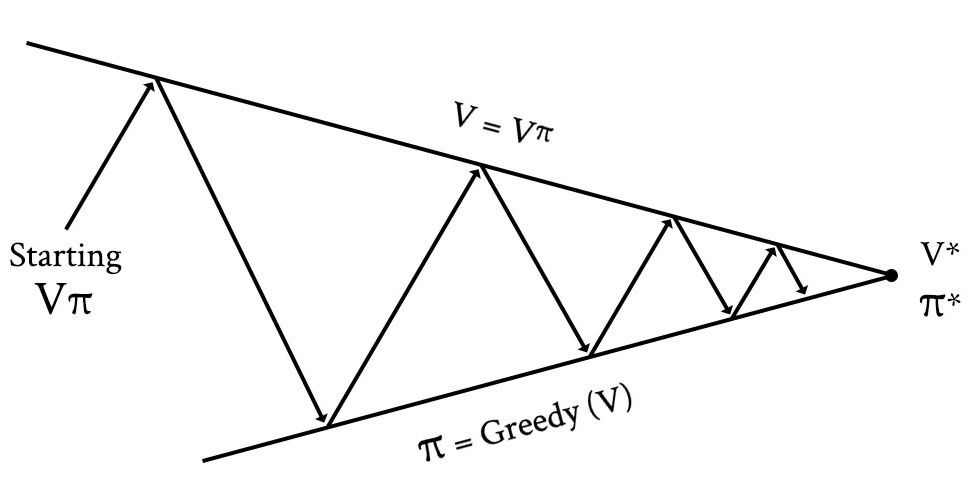
The challenge of circular dependencies and stochastic probabilities can be addressed by calculating state-values iteratively. That is, we run our agent through the environment many, many times, calculating state-values along the way, with the goal of improving the accuracy of the V and/or Q each time. Using this approach, the agent is first provided with an initial policy. This default policy might be totally stupid (e.g., choose actions at random) or based on an existing policy that is known to work well. Then, the agent follows this policy over and over, recording the state-values (and/or action-values) with each iteration. With each iteration, the estimated state-values (and/or action-values) become more and more accurate, converging toward the optimal state-value (_V*_) or the optimal action-value (_Q*_). This type of iteration solves the chicken-or-the-egg problem of calculating estimated state-values with circular dependencies. Updating estimated state-values this way is called “prediction” because it helps us estimate or predict future reward.
While prediction helps refine the estimates of future reward with respect to a single policy, it doesn’t necessarily help us find better policies. In order to do this, we also need a way to change the policy in such a way that it improves. Fortunately, iteration can help us here too. The process of iteratively improving policies is called “control” (i.e., it helps us improve how the agent behaves).
Reinforcement learning algorithms work by iterating between prediction and control. First they refine the estimate of total future reward across states, and then they tweak the policy to optimize the agent’s decisions based on the state-values. Some algorithms perform these as two separate tasks, while others combine them into a single act. Either way, the goal of RL is to keep iterating to converge toward the optimal policy.

Exploration vs. Exploitation
But before we can start writing a reinforcement learning algorithm, we first need to address one more conundrum: How much of an agent’s time should be spent exploiting its existing known-good policy, and how much time should be focused on exploring new, possibly better, actions? If our agent has an existing policy that seems to be working well, then when should it wander off the happy path to see if it can find something better? This is the same problem we face on Saturday night when choosing which restaurant to go to. We all have a set of restaurants that we prefer, depending on the type of cuisine we’re in the mood for (this is our policy, π). But how do we know if these are the best restaurants (i.e., π*)? If we stick to our normal spots, then there is a strong probability that we’ll receive a high reward, as measured by yumminess experienced. But if we are true foodies and want to _maximize_ future reward by achieving the _ultimate_ yumminess, then occasionally we need to try new restaurants to see if they are better. Of course, when we do this, we risk experiencing a worse dining experience and receiving a lower yumminess reward. But if we’re brave diners in search of the best possible meal, then this is a sacrifice we are probably willing to make.
RL agents face the same problem. In order to maximize future reward, they need to balance the amount of time that they follow their current policy (this is called being “greedy” with respect to the current policy), and the time they spend exploring new possibilities that might be better. There are two ways RL algorithms deal with this problem. The first is called “on-policy” learning. In on-policy learning, exploration is baked into the policy itself. A simple but effective on-policy approach is called ε greedy (pronounced epsilon greedy). Under an ε greedy policy, the policy tells the agent to try a random action some percentage of the time, as defined by the variable ε (epsilon), which is a number between 0 and 1. The higher the value of ε, the more the agent will explore, and the faster it will converge to the optimal solution. However, agents with a high ε tend to perform worse once an optimal policy has been found, because they keep experimenting with suboptimal choices a high percentage of the time. One way around this problem is to reduce or “decay” the value of ε over time, so that a flurry of experimentation happens at first, but occurs less frequently over time. This would be like going to many new restaurants after you first move into a new town, but mainly sticking to the tried-and-true favorites after you’ve lived there for a few years.
Another approach to the exploration-versus-exploitation problem is called “off-policy” learning. Under this approach, the agent tries out completely different policies, and then merges the best of both worlds into its current policy. In off-policy learning, the current policy is called the “target policy,” and the experimental policy is called the “behavior policy.” Off-policy learning would be like occasionally following the advice of a particular food critic from your local paper, and then trying all the restaurants she likes for a while as a means of discovering better dining options.
RL Algorithm: Q-Learning
Q-learning is a popular, off-policy learning algorithm that utilizes the Q function. It is based on the simple premise that the best policy is the one that selects the action with the highest total future reward. We can express this mathematically as follows:

This equation says that our policy, π, for a given state, s, tells our agent to always select the action, a, such that it maximizes the Q value.
In Q-learning, the value of the Q function for each state is updated iteratively based on the new rewards it receives. At its most basic level, the algorithm looks at the difference between (a) its current estimate of total future reward and (b) the estimate generated from its most recent experience. After it calculates this difference (a – b), it adjusts its current estimate up or down a bit based on the number. Q-learning uses a couple of parameters to allow us to tweak how the process works. The first is the learning rate, represented by the Greek letter α (alpha). This is a number between 0 and 1 that determines the extent to which newly learned information will impact the existing estimates. A low α means that the agent will put less stock into the new information it learns, and a high α means that new information will more quickly override older information. The second parameter is the discount rate, γ, that we discussed in the last article. The higher the discount rate, the less important future rewards are valued.
Now that we’ve explained Q-learning in plain English, let’s see how it’s expressed in mathematical terms. The equation below defines the algorithm for one-step Q-learning, which updates Q by looking one-step ahead into the future when estimating future reward. Below is the annotated equation for Q-learning:

But we can simplify the annotated explanation of the equation even further. At its most basic level, Q-learning simply updates the existing action-value by adding the difference between the old estimate of future reward and the new estimate, multiplied by the learning rate:

One-step Q-learning is just one type of Q-learning algorithm. DeepMind used a more sophisticated version of Q-learning in its program that learned to play Atari 2600 games. There are also other classes of reinforcement learning algorithms (e.g., TD(λ), Sarsa, Monte Carlo, FQI, etc.) that do things a little differently. Monte Carlo methods, for example, run through entire trajectories all the way to the terminating state before updating state- or action-values, rather than updating the values after a single step. Monte Carlo algorithms played a prominent role in DeepMind’s AlphaGo program.
Dealing with insanely large state spaces
This is all well and good, but the reinforcement learning techniques we’ve discussed thus far have made a critical underlying assumption that doesn’t hold true very often in the real world. So far, we’ve implicitly assumed that the MDP we’re working with has a small enough number of states that our agent can visit each state, many, many times within a reasonable period of time. This is required so that our agent can learn the underlying probabilities of the system and converge toward optimal state- and/or action-values. The problem is that state spaces like Go, and most real-world problems, have a ginormous number of states and actions. Our agent can’t possibly visit every state multiple times when, as is the case with Go, there are more states than there are atoms in the known universe — this would literally take an eternity.
In order to overcome this problem, we rely on the fact that for large state spaces, being in one state is usually very closely correlated to being in another state. For example, if we are developing a reinforcement learning algorithm to teach a robot to navigate through a building, the location of the robot at state 1, is very similar to the location of the robot at state 2, a few millimeters away. So, even if the robot has never been in state 2 before, it can make some assumptions about being in that state based on its experience being in other nearby states.
In order to deal with large state spaces, we use a technique called “function approximation.” Using function approximation, we approximate the value of V or Q, using a set of weights represented by θ (theta), that essentially quantify which aspects of the current state are the most relevant in predicting the value of V or Q. These weights are learned by the agent automagically through a completely different process. This new process works by logging the reward that the agent receives as it visits the various states, and storing this experience in a separate dataset. Each row of this new dataset records the state the agent was in, the action it took in that state, the new state the agent ended up in, and the reward it received along the way. What’s interesting about this “experience” dataset, is that it is essentially a supervised learning training dataset (which we touched on briefly in the last article). In this RL experience dataset, states and actions represent features that describe observations, and rewards represent the labeled data that we want to predict. In essence, by taking action in the world (or in a simulated version of the world), RL agents generate their own labeled training data through their experience. This training data can then be fed into a supervised learning algorithm to predict state-values and/or action-values when the agent arrives at a state it hasn’t visited before. The supervised learning algorithm then adjusts a set of weights (θ), during each iteration, refining its ability to estimate V and Q. These weights then get passed into the V and Q functions, enabling them to predict cumulative future reward.
With this clever little trick in hand, we can now leverage the huge amount of research that has gone into predictive, supervised learning and use any of a number of well-documented algorithms as our function approximator. Although just about any supervised learning algorithm will work, some are better than others. The folks at DeepMind were smart, and they chose an algorithm for their function approximator that has been killing it recently in the area of machine vision — deep neural networks. In the next article, I’ll provide an overview of how artificial neural networks (ANNs) work and why deep neural networks in particular are so effective. Deep learning is a red hot topic right now, and the success of AlphaGo poured flame on the fire. Neural networks and deep learning are a bit more difficult to understand than reinforcement learning, but we’ll continue to unpack the algorithms in a way the surfaces the intuition behind the math. Despite the fact that the terminology of deep learning sounds like neuroscience, it is still just a souped-up algorithm — not a human-like-brain implemented in silicon.
Further Exploration:
- DeepMind’s paper in Nature on the program that learned 49 Atari games
- DeepMind’s paper in Nature on AlphaGo
- David Silver’s class on reinforcement learning, published by Google
- Barto and Sutton’s textbook on reinforcement learning, considered the Bible of RL