
The focus of this series is to dissect the methods used by DeepMind to develop AlphaGo, the machine learning program that shocked the world by defeating a worldwide Go master. By peeking under the hood of DeepMind’s algorithm, we hope to demystify Machine Learning (ML) and help people understand that ML is merely a computational tool, not a dark art destined to bring about the robot apocalypse. In the earlier articles we discussed why AlphaGo’s victory represents a breakthrough, and we explained the concepts and algorithms behind reinforcement learning—a key component of DeepMind’s program. In this article, we’ll explore artificial neural networks. Neural networks form the foundation of deep learning, the technique that enabled DeepMind’s reinforcement learning algorithm to solve extremely large and complex problems like Go. Deep learning is an advanced form an artificial neural network. So, before we dive into deep learning in the next article, we’ll first explore how a neural network operates.
Neural networks were conceived in the middle of the twentieth century as scientists started understanding how the brain works. What makes the brain so interesting to computer scientists is that in many ways it acts like a mathematical function: input comes in (in the form of electrical and chemical signals), some type of neurological computation happens, and output goes out to other cells. For example, you receive input from your sensory system, perhaps noticing a burning sensation on your hand. Then your brain performs some computation, such as determining that your hand has touched a hot pan. Finally, electrical output is sent to your nervous system causing you to contract your arm muscles and jerk your hand away from the hot surface.
In the 1940s and 50s a group of scientists, including Warren McCulloch, Walter Pitts and Frank Rosenblatt published a series of papers that laid out the blueprint for the first algorithms based on the brain. They observed that the brain is a network, made up of billions of nerve cell connectors called neurons. Neurons are comprised of branch-like receptors called dendrites, that receive electrical impulses from other upstream neural cells, and a long, thin projection called an axon that sends signals downstream to other neurons. Once a neurons’ dendrites receive an impulse, if a certain threshold is reached, the neuron fires and it sends a signal to other neurons through its axon. Since neurons are connected in a large network, when an impulse is received by one neuron, it can set off a wide range of electrical activity within the brain, creating a chain reaction.
 Neuron - Source: Wikipedia / Creative Commons
McCulloch, Pitts and Rosenblatt realized that a simplified version of this neurological process could be used to implement a self-learning computer function. They understood that the brain is able to update the strength of its neural connections automatically over time as it gains new experience, and that these neural adjustments are how people learn concepts and store memory. Based on this “connectionist” approach, they pioneered a completely new approach to computer science.
The Small but Mighty Perceptron
Rosenblatt’s artificial neuron, the perceptron, was a popular early implementation of this neurological architecture. The perceptron was designed to be a simple electronic representation of a single neuron. Like a real neuron, it received input, performed a calculation and “fired” if a certain threshold was met. In addition, it updated its connection strength based on its experience, and thus was able to “learn” from experience. Although relatively simple by today’s standards, the perceptron still forms the basis for a class of powerful prediction algorithms. For example, we could use the perceptron to create a program to detect fraudulent credit card transactions. We would do this by compiling a large list of existing transactions that we know to be either legitimate or fraudulent, and feeding the dataset to the perceptron to learn to predict fraud.
The perceptron algorithm takes a series of numbers as inputs and runs them through a set of corresponding numerical weights. The inputs are analogous to a neurons’ dendrites receiving electrical impulses, the weights represent the connection strength between neurons, and an activation function determines if the threshold has been reached. (Fancier options for the activation function came later, but the original perceptron used a very simple activation function called a step function that simply returned 1 if net input is above the threshold, or 0 otherwise.)
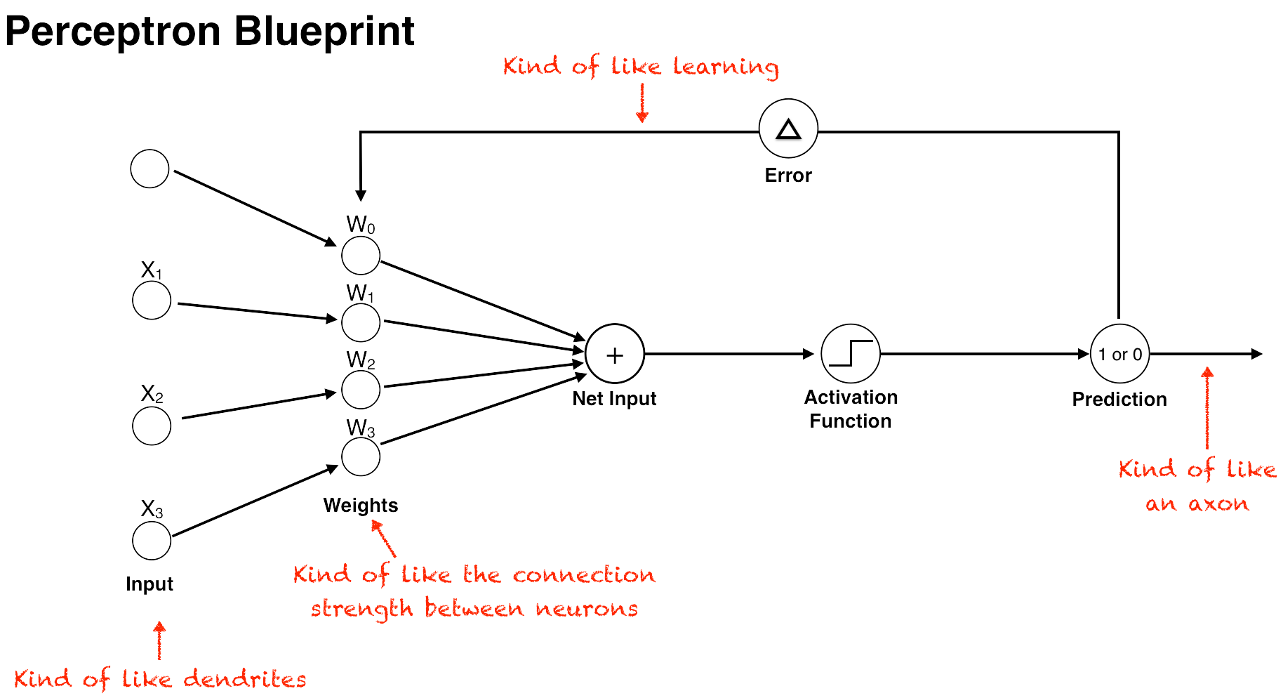
In the perceptron algorithm, the inputs are multiplied by their corresponding weights, and the results of these products are added up. The resulting number, the net input, is then checked against the threshold. If it’s above the threshold, then the perceptron “fires” and outputs a 1, otherwise it outputs a 0 (this is called the Step function).


The secret sauce of the perceptron, however, is not the method by which it calculates an output, but how it learns from its mistakes and updates its weights to improve performance. It does this by first comparing its output (a 1 or 0) against the actual outcome in the training data. Next, it subtracts its predicted outcome from the real outcome—the difference representing the training “error.” Then, it multiplies the error by a learning rate (a number between 0 and 1) that determines the extent to which new information should impact the existing weights. A low learning rate means less stock will be put into the new information it learns, and a high number means that new information will more quickly override older information. (This similar to the learning rate we discussed in the Q-Learning algorithm in the last article.) The resulting number represents the amount the weights should be adjusted, or the “change-in-weights.”


Finally, the perceptron adds the change-in-weights to each one of the existing weights, and the perceptron now has an updated set of weights that yield a more accurate outcome. This is how the perceptron learns, by using its weights to try to calculate an outcome, checking the outcome against the actual result, and adjusting its weights accordingly. The more training data the perceptron is fed, the more this process repeats itself, and the more accurate the perceptron’s output becomes.

Now that we understand how the perceptron works, let’s see how it could be used to implement our credit card fraud detection system. First, we would need to compile a large list of transactions that we already know are either legitimate or fraudulent. This dataset would have one row per transaction, and it would contain several columns that quantitatively describe each transaction, such as the transaction amount, time of transaction, transaction location, number of transactions within the last 24 hours, etc. These columns are called “features” in ML parlance and the rows are called “samples,” “training examples,” or “observations.” The known outcome (fraud or not) for each transaction is called the “label.” The features would be used as the inputs for our perceptron (in actuality, the original perceptron only accepted binary input—a 1 or 0—but modern-day neural networks can accept any old number). Then, we would let the perceptron’s output represent the outcome we are trying to predict, a 1 if the transaction is fraudulent, 0 if it’s legit.

Within our fraud detection system, the weights of the perceptron would represent how much each feature counts toward the prediction. For example, if one of our features was “phase of moon on transaction day,” this probably wouldn’t help much in predicting fraud, and would therefore have a correspondingly low weight. On the other hand, the feature “number of transactions within 24-hours” would probably be a strong factor in determining fraudulent activity, and thus its input would have a much larger weight. With our large dataset of labeled transactions, then, we could simply feed the data to the perceptron, update the weights as we run through each row, and end up with a decent model for predicting fraud. Machine intelligence achieved, right?
Trouble in AI Paradise
Well, not exactly. Although the perceptron represented a huge advancement in AI, it suffered from a couple of big problems. First, the process used for predicting the outcome—i.e. using a weighted sum of the inputs—is a form of a linear equation. Linear equations are a type of function that output a line. In the case of the perceptron, the linear equation is used to draw a boundary between the classes it is trying to predict. For example, transactions that are fraudulent would fall above the line, and those that aren’t would fall below it. While many classification problems can be predicted using linear equations, many more cannot. So the fact that the perceptron’s predictions are based on a linear equation means it is limited in the types of problems it can address.
 Linear Classifier
A symptom of this problem is the fact that the perceptron can’t implement an “Exclusive Or” (XOR). XOR is a simple logic function that returns true if either of its two inputs are true, but not if both are. Pedro Domingos provides a good example of XOR in his book The Master Algorithm. Nike is said to be popular among teenage boys and middle-aged women. Therefore, people who are female or young, may be receptive to a Nike advertisement, but those who are female and young, are a much less attractive prospect. Furthermore, if you are neither young nor female, you’re also an unpromising prospect. If you were using a perceptron to build a targeted marketing engine, you wouldn’t be able to handle this type of relationship.
| Female | Young | Strong Sales Prospect? |
|---|---|---|
| 0 | 0 | No |
| 1 | 0 | Yes |
| 0 | 1 | Yes |
| 1 | 1 | No |
| XOR Logic Table |
Making matters worse, implementing XOR—a fundamental logic function—is trivial using traditional computer science approaches, yet is impossible to do with a perceptron. Theoretically, it was possible to solve XOR with a perceptron using multiple layers of inputs and weights. Such a multilayer perceptron (MLP) would contain an input layer, one or more intermediate hidden layers, and an output layer. (The middle layers are called the “hidden” layers because we don’t see the output of their calculations—they are fed into other intermediate layers or to the output layer directly.) Under this scenario, a network of three neurons in two layers could solve our Nike example. One neuron could fire when it receives input indicating a young male, another when it sees a middle-aged woman, and the third fires if either of the other nodes fire.
") Stacking neurons together in a multilayer perceptron (MLP)
Stacking neurons together in a multilayer perceptron (MLP)
Although a multilayer perceptron looked promising on paper, at the time, it was considered impractical to implement due to something called the credit assignment problem. In a system with multiple layers of interconnected nodes, how do we know which nodes contributed to what degree to a prediction error? That is, how do we assign credit to the nodes that contributed the most to the prediction? This was easy to do with a single layer perceptron, but devilishly hard when additional layers are introduced.
For academics in the competing “symbolist” camp of AI, the weakness of the perceptron was simply too good to pass up. Smelling blood in the water, in 1969 AI luminary and symbolist ring leader Marvin Minsky co-authored a book with Seymour Papert called Perceptrons that laid out a searing indictment of the perceptron. The book turned out to be enormously influential, and dealt a huge blow to the connectionists. In fact, the book was so influential that it caused a freeze on the research of neural networks for 15 years—a period that came to be known as the “AI Winter.”
The Neural Network Strike Back
Despite the fallout from Perceptrons, work on neural networks continued behind the scenes and three major advances were made that started to address the shortcomings of the early neural networks. First, instead of using the output of the step function (which returned 1 or 0) to calculate the prediction error, the output of the net input was used directly. This was a big improvement because net input is a continuous value (that is, it could be any Real number) not a just binary one, which means it generates much more granular feedback. Simply relying on the output of “the prediction was right” or “the prediction was wrong” doesn’t give us much to go on when adjusting our weights. By using net input instead, we could now update the weights based on how close it was to getting it right.
A second and related improvement is that by using the continuous-valued net input function directly as our activation function, it now produces a silky smooth line, instead of the herky jerky line created by the step function. This gave the function an important mathematical property: it made it differentiable. Differentiability is a concept from Calculus that denotes a function that produces a line that is smooth, continuous and predictable. This predictability is a good thing because it means we can use a bit of Calculus to more effectively find the optimal weights, using a technique called gradient descent.
Gradient descent is an important technique in machine learning. Gradient descent is an algorithm used to minimize a cost function. What’s a cost function? A cost function simply measures how far away a machine learning model is to finding the optimal solution. In the case of a neural network, the cost function is just our error function that calculates the difference between the predicted outcome and the actual value. Gradient descent is the mathematical equivalent of walking down a hill in a dense fog, step by step, using the decline of the hill to guide our way down. Using gradient descent, we slowly walk down the “error” hill, tweaking the weights as we go, until we find the lowest point which represents the smallest error (and thus the best possible predictor). Calculus gives us some special tools (namely, derivatives) that allow us to calculate the rate at which the cost changes in relation to our weights, and this gives us the ability to find the slope downhill (i.e. the gradient) in the fog.
The third, and perhaps most important advancement to happen during this time was the discovery of Backpropagation. Backpropagation is a powerful technique used to solve the credit assignment problem in a multilayer perceptron. Backpropagation uses another bit of Calculus (a method called the Chain Rule) that allows us to work backward through each layer in the network to find the gradient of each node. Using this technique, we first put some training data through our multilayer neural network and predict an outcome based on our weights, just like normal. This is called forward propagation. Then, we check our output, calculate the prediction error, and walk back through each layer of network using backpropagation to calculate the gradient for each node. Since the gradient tells us the direction our weights should be adjusted to make the prediction more accurate, using Backpropagation we can micro tweak the weights of each node in each layer to make it a little more accurate without unintentionally causing the whole network to become unstable.
 Backpropagation
Deep Learning Emerges
In 1986, Geoffrey Hinton, David Rumelhart and Ronald Williams, published a paper called “Learning representations by back-propagating errors” that broke the logjam for neural network research. In the paper, they unveiled Backpropagation and made a compelling case for why it solved the seemingly intractable problem of credit assignment in multilayer perceptrons. As a result of their work, the long freeze of the AI Winter finally came to an end, and the enormous potential of neural networks seemed possible once again. Another consequence of the paper was the emergence of Geoffrey Hinton as the preeminent leader of the connectionists. Hinton (who now works for Google, in addition to teaching) went on to become one of the most prolific contributors to the study of neural networks and has come to be known as the grandfather of deep learning.
So, despite the somewhat obtuse, biologically-inspired terminology of neural networks, at its core an artificial neuron is pretty basic. It’s just a series of inputs and weights that produce an output if the sum of their products reaches a certain threshold. By taking the difference between the calculated output and the actual output, we can then adjust the weights slightly to make our output a little more accurate each time. With the use of techniques like backpropagation, we can then connect multiple layers of neurons together in a network to solve more complex problems. However, despite the fact that neural networks were inspired by the brain, in reality, they are more like a child’s stick figure representation of it—the human brain is vastly more complex. And although a neural network can perform some pretty amazing tasks, at the end of the day it is still just a plain old computational algorithm—not the birth of self-conscious AI.
In the next article will see how neural networks have evolved into deep learning, and how DeepMind used these advances to build their Go-conquering program.
Further Exploration:
- Andrey Kurenkovs’ blog posts on the history of neural networks and deep learning.
- The Master Algorithm – A great book by University of Washington professor Pedro Domingos that provides a survey of machine learning approaches in a quest to find the single algorithm to rule them all.
- Stanford’s CS231n course on deep learning, with Andrej Karpathy.
- Michael Nielsen online book on neural networks and deep learning.
- DeepLearning TV’s introductory video series to Deep Learning. Very visual. No math.
- Sebastian Raschka’s blog post on early neural networks and gradient descent.
- Sebastian Raschka’s book, Python Machine Learning, which explains how to implement neural networks and other ML algorithms in Python.