In the first article in this series, we discussed why AlphaGo’s victory over world champ Lee Sedol in Go represented a major breakthrough for machine learning (ML). In this is article, we’ll dissect how reinforcement learning (RL) works. RL is one of the main components used in DeepMind’s AlphaGo program.
Reinforcement Learning Overview
Reinforcement learning is a subset of machine learning that has its roots in computer science techniques established in the mid-1950s. Although it has evolved significantly over the years, reinforcement learning hasn’t received as much attention as other types of ML until recently. To understand why RL is unique, it helps to know a bit more about the ML landscape in general.
Most machine learning methods used in business today are predictive in nature. That is, they attempt to understand complex patterns in data — patterns that humans can’t see — in order to predict future outcomes. The term “learning” in this type of machine learning refers to the fact that the more data the algorithm is fed, the better it is at identifying these invisible patterns, and the better it becomes at predicting future outcomes.
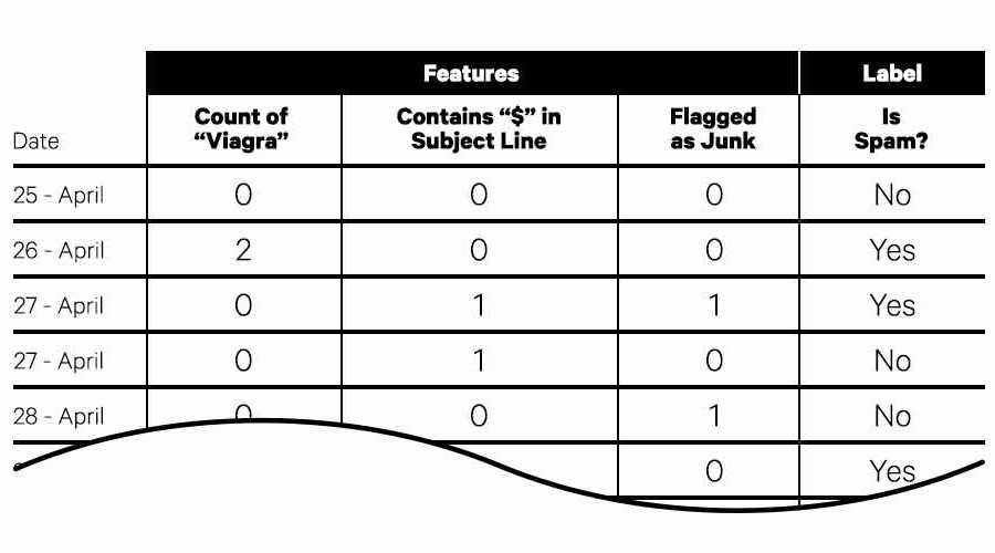
This type of predictive machine learning falls into two categories: supervised learning and unsupervised learning. Supervised learning uses large sets of training data that describe observations that have occurred in the past. This training data contains columns that quantitatively describe the observations (these descriptive columns are called “features”), in addition to the final outcome of the observation that the algorithm is trying to predict (this is called the “label”). For example, a spam filter designed to predict if an incoming email is spam might look at millions of emails that have already been classified as spam or not-spam (this is the label) to learn how to properly classify new emails. The list of existing emails are the observations (also called “samples”). The features in the dataset might include things like a count of the word “Viagra” in the text of the email, whether or not the email contains a “$” in the subject line, and the number of users who have flagged it as junk email.

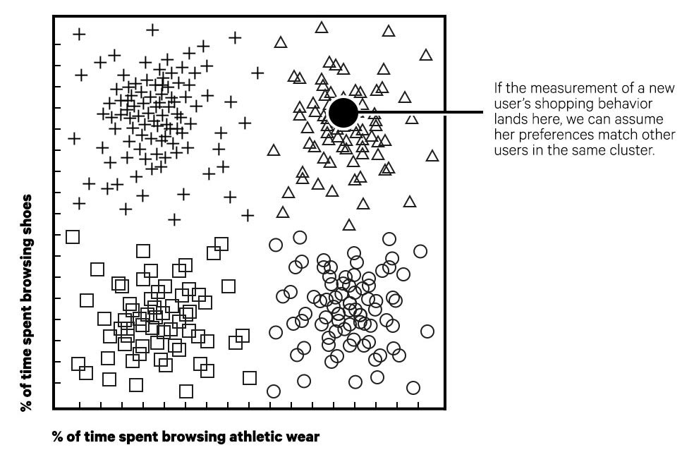
The other category of predictive machine learning is unsupervised learning. Unsupervised learning attempts to find hidden patterns and structures in data on its own, without relying on labeled training data. In some cases, unsupervised learning can be used to pinpoint which features matter the most. In other cases, it uses features to cluster similar types of items based on correlations between their characteristics. The classic example of unsupervised learning is an e-commerce recommendation engine. For example, let’s say you had millions of observations of people shopping on a women’s apparel e-commerce site. You could use the feature data to identify clusters of shoppers with similar preferences, such as women who prefer specific brands, as measured by their purchasing history. Then, when a new customer starts using the site, you could use the items she browses as a set of features and use this to identify the cluster of shoppers she is most similar to (as measured by her distance to the nearest cluster when plotted on a chart). From there you could get a list of items purchased by other people in the cluster and use this as the basis for recommending products to the new shopper. This is a simple unsupervised learning algorithm called “k Nearest Neighbors.”

Reinforcement learning, however, is different in kind from predictive ML. Supervised and unsupervised learning methods are “one-shot” classifiers that attempt to make a single prediction from the data (given a set of features X, the most likely outcome is the value Y). RL, in contrast, is designed to implement higher order cognitive thinking. Specifically, RL seeks to find optimal decisions that benefit the user over the long term, even if this requires taking undesirable actions in the short term. For example, in a down market, it may be beneficial to sell a stock at a loss in the short term, in order to use that capital to purchase a bond that has a better chance of yielding a return in the long run.
Reinforcement learning is neither supervised nor unsupervised. Instead, in RL a computer agent learns by interacting directly with its environment (or a simulated version of its environment) and recording the reward it gets along the way. The goal of an RL agent is simply to identify those actions that will lead to the maximum, cumulative future reward. This approach is similar to the way the brain uses dopamine as a signal to guide animal and human behavior.
Because the RL agent learns directly from its environment, it doesn’t require huge amounts of pre-existing, domain-specific, training data to learn. Rather, it generates its own training data simply by interacting with its environment and learning from its experience. This approach enables RL to serve as a general purpose learning algorithm. Whereas predictive ML uses heavily curated, domain-specific, pre-existing data for learning, an RL agent learns from its own experience, much like a young child does. If you place the RL agent in an environment where the goal is to win Asteroids, it will learn how to play Asteroids. If you place the agent in an environment where the goal is to go from point A to B, then you can teach a robot to navigate through a warehouse. You do have to create a mapping that translates the environment and the reward signal for a specific domain into a common structure that an RL agent understands (and this is not always trivial), but the underlying decision-making algorithm can be substantially the same across domains. This explains how DeepMind was able to use the same algorithm with the same hyperparameters (these are the high-level knobs used to tune the system) to learn 49 different Atari games each with very different rules, game mechanics and scoring systems. This type of general learning approach stands in stark contrast to DeepBlue (the machine that IBM built to beat Grandmaster Garry Kasparov at Chess) which was purpose-built to play Chess.
The Components of a Reinforcement Learning System
With a general understanding of reinforcement learning in place, now we’ll dig a little deeper to understand how RL algorithms work under the hood. There are several different types of RL algorithms, but they all make use of the same system of components:
Agent: This is the machine doing the learning. The agent is the program running on a processor (or cluster of processors) that implements the RL algorithm.
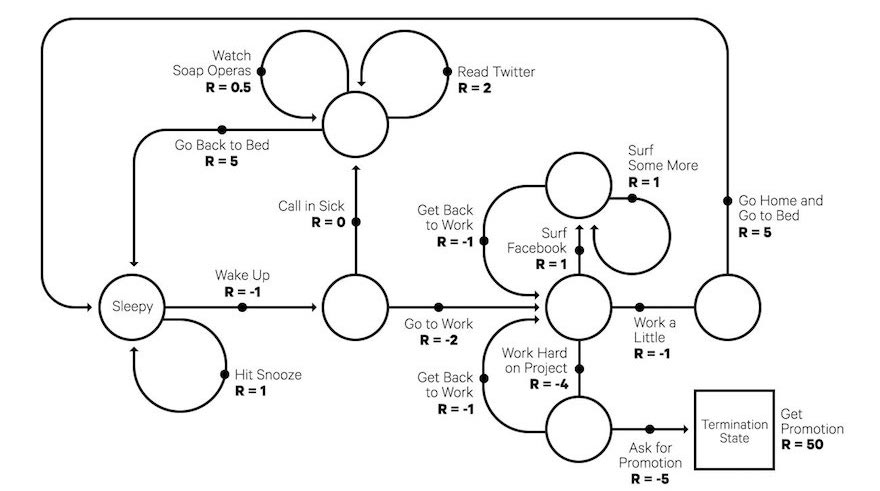
Environment: This is the digital representation of the world in which the agent operates. Classically, RL problems are represented by a Markov Decision Process (MDP). An MDP is like a flow chart with circles representing each state, and arrows jutting out from each circle that represent all the possible actions that can be taken from that state. For example, an MDP representing a Chess game would have states that represent where all the pieces on the Chess board are located, and actions representing the possible moves based on the Chess pieces on the board.
 A simple Markov Decision Process (MDP) that represents a typical workday
A key characteristic of an MDP is that each state must contain all the information the agent needs in order to make an informed decision, a requirement called the “Markov property.” The Markov property basically says that the agent can’t be expected to have any historical memory of its own, outside the state itself. For example, the current state of the Chess board tells me everything I need to know about which is the best move to make next — I don’t need to remember the moves that were made prior in the game. In practice, the real-world problem you are trying to model doesn’t have to be perfectly Markov in order for RL to be able to solve the problem. For example, my memory of how a particular opponent plays Chess may factor into my decision-making process in the real world, but I can still make a winning Chess playing agent with RL that ignores this information. However, if there are pieces of information that are relevant to solving the problem, then they often can be quantified and included as part of the state itself.
Reward: RL agents learn by analyzing the reward signal in their environment. The agent’s goal is to maximize the total, cumulative, future reward over the long term. Although RL works very well when reward signals are frequent (e.g., video game scoring or the financial return from stock trading), it also works when reward signals are infrequent (e.g., winning or losing a 4-hour Go match).
Action: In each state, the agent is presented with a number of possible choices. For a stock trading agent, the choices might be buying more shares of a given company, selling some of the shares, or holding the stock. The goal of the agent is to learn the best action to take in its current state. In some environments, like Go or Chess, the result of each action is deterministic. That is, if the agent selects a valid action, the result of that action will always be the same. For example, if the agent makes a valid move in Go, the piece always lands in the intended spot. But life is not always this simple. In other environments, such as medical diagnosis, the actions are stochastic, which means they are determined somewhat randomly. For example, if a doctor chooses to give a patient treatment A (the action), given a particular diagnosis B (the state), and there is an 80% chance the treatment will cure the disease (the probability of getting to the state C, curing the patient), then the doctor is working in a stochastic environment. Fortunately for us, reinforcement learning is designed to accommodate both deterministic and stochastic environments.
Policy: A policy simply tells the agent which action to take when they find themselves in a given state. The policy is represented in RL equations by the Greek letter pi (π). The purpose of RL is to learn the best policy, and RL algorithms provide the blueprint to tell the agent how to find it. For simple problems, it is possible to mathematically calculate the optimal policy. This is denoted as π* (pronounced “pi star”). For most real-world problems, however, it’s not feasible to find π*. Instead, we pursue a more realistic objective of continuously improving the policy so that it converges toward π*, even if we can’t find the optimal policy precisely.
Discount Rate: For many types of RL problems, the value of a reward in the future is less than the value of a reward right now. For example, in finance, a dollar in my hand today, is worth more than a dollar in my hand a year from now (this is called the time value of money). This concept is represented in RL as the discount rate, which is denoted by the Greek symbol gamma (γ). The discount rate is a number between 0 and 1 that determines exactly how much less a reward earned in the future is worth, compared to a reward earned immediately. The lower the discount rate, the less the future reward is worth. The total, discounted future reward (called the Discounted Return, or R) can be represented mathematically as follows:

This equation simply says that the Discounted Return, R, at time t, equals a sum of all future rewards, r, and that rewards earned in future time periods are reduced by multiplying the reward by the discount rate , which is typically some fractional number between 0 and 1 (e.g. 0.5). The mathematical trick used to amplify the discount as the rewards get farther into the future (and thus reducing the reward), is to add an exponent on it (e.g., γ2) that increases at each step in the future.
State-Value Function: In reinforcement learning, the value of the total estimated future reward in a given state is determined by a special function called the “state-value function,” represented as V. The state-value function works by calculating the total estimated future reward that would be earned by visiting each state in the future when following policy, π until reaching the terminating state. The terminating state (also called the “absorbing state”) might be the end of a game or just a distant point in the future. We can represent V mathematically as follows:

This equation basically says that the state-value of a given state, when we’re following policy π, is the sum of all future rewards from that point forward, taking into account probabilities (if the environment is stochastic) and our discount rate. Just as there is an optimal policy ( π* ), there is also an optimal value function, V*. For large state spaces, we may never be able to find V* precisely, but we should be able to converge toward it with the right RL algorithm.
Action-Value Function: The mathematical sister of the state-value function is the action-value function, represented as Q. Whereas the state-value function is concerned with determining the total future reward of each state, the action-value function seeks to determine the total future reward of each state/action pair. Although both functions accomplish a similar objective, they are used in different ways in different RL algorithms. The equation for the action-value function is below. It is the substantially same as, V, except that it is calculated for state, s, and action, a.

Just as there is an optimal state-value function, there is also an optimal action-value function, represented as Q*.
Summary
Although the math behind machine learning does an excellent job of describing algorithms in precise terms, it can also obfuscate the intuitive nature of these algorithms for non-mathematicians. This is unfortunate, because by making machine learning difficult to comprehend, it also makes it appear more like black magic to the general public, which in turn creates a mood of fear and confusion. The reality is, however, that machine learning is just another evolution in computer programming — not the birth of sentient artificial intelligence. While it is certainly true that machine learning is starting to solve much more complex problems than we have been able to do so in the past, this is a far cry from the beginning of robot domination.
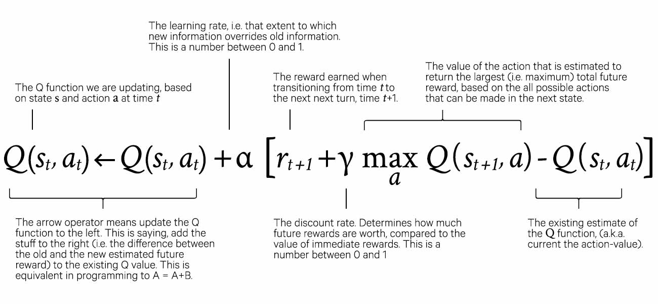
The reinforcement learning algorithm at the heart of DeepMind’s program is a case in point: although its potential to solve problems is impressive, its inner workings are fairly easy to grasp. At its most basic level, reinforcement learning is the computer equivalent of training a rat to run through a maze by rewarding it with cheese at the end. By running the rat through the maze over and over, it quickly learns the fastest way through the maze. Instead of using a maze, however, reinforcement learning uses a Markov Decision Process with states and actions, and instead of using cheese as a reward, RL agents follow a numerical reward signal. In this article we have described these components — the parts that make up an RL system — but we haven’t yet examined how they come together in an RL algorithm. In the next article, we’ll dissect the Q-Learning RL algorithm to understand how these components are combined to solve very difficult problems.
Further Exploration:
- DeepMind’s paper in Nature on the program that learned 49 Atari games
- DeepMind’s paper in Nature on AlphaGo
- David Silver’s class on reinforcement learning, published by Google
- Barto and Sutton’s textbook on reinforcement learning, considered the Bible of RL